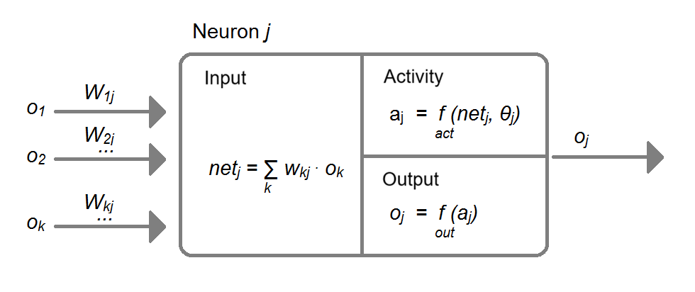
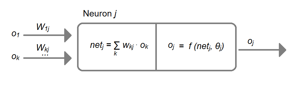
The basic structure of an artificial neuron corresponds to that of its biological counterpart and is replicated in the form of software modules:
An artificial neuron receives input information via connections to other neurons with corresponding input values Ok, where k = 1..n.
The influence of these input values is modelled by n real numbers, referred to as input weights Wkj (corresponding to synapses in the biological world).
|
The propagation functionj combines the inputs with the weights and aggregates the overall information. The activation function determines the new activity aj using a threshold θj. The output function fout determines the output value oj from the neuron’s activity aj.

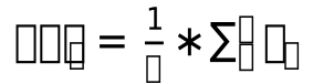
The propagation function is often referred to as the netj input and forms the basic element of the neuron. To obtain a uniform average value across all inputs, the arithmetic mean would be the obvious choice:
|
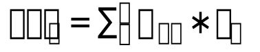
In order to take account of the varying influence of the individual inputs, each input ok is assigned a weight wkj and a weighted average is calculated. The normalisation factor 1/n is usually multiplied by the activation or output function. This simplifies the propagation function as follows:
|
Most neuron models use this type of network input or propagation function.
The activation function of an artificial neuron determines how the activity is calculated from the output value of the propagation function. A wide variety of functions can be used as activation functions.
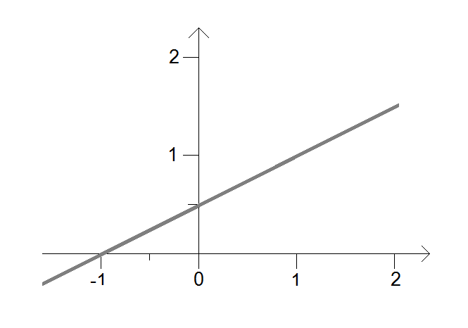
The simplest activation function is the linear function, which is characterised solely by a threshold value and a slope. The range of values for the activity level is unbounded in both directions.
Linear function
The linear function is described by the following formula:

|
|
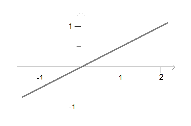
Linear function with a threshold of zero
The formula can be simplified by setting the threshold to zero:

|
|
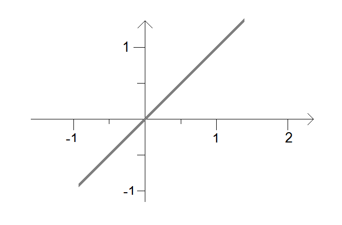
Identity
The slope can also be set to one, resulting in the identity as the activation function:

|
|
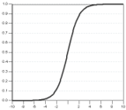
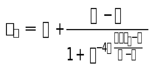
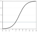
The Fermi function, also known as the logistic function, is a typical monotonically increasing function and is frequently used in neural networks. The simple Fermi function is a special case of the general Fermi function with the parameters m=0, M=+1, θ=0 and σ=0.25.
Simple Fermi function
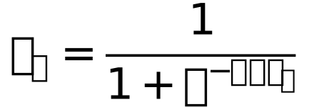
The range of this function lies in the interval (0,1). The simple Fermi function is given by the formula:
|
|
General Fermi function
The slope of the General Fermi function is determined by the parameter σ. The function is given by the formula:
|
|
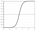
The hyperbolic tangent (tanh) is also very commonly used as an activation function. With both the logistic function and the hyperbolic tangent, the activity level is bounded above and below. As a result, the activity level remains restricted to a narrow range of values (e.g., from -1 to 1 for the hyperbolic tangent function). Due to this limited range, these functions are frequently used as activation functions for the neurons in the hidden layers (while other activation functions are often used for the neurons in the output layer).
Hyperbolic Tangent
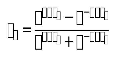
The hyperbolic tangent is also a special case of the general Fermi function with the parameters m=-1, M=+1, θ=0, and σ=1. The hyperbolic tangent is described by the following formula:
|
|
The linear, logistic, and hyperbolic tangent functions are differentiable at all points; that is, a derivative can be computed at every point. Differentiability is a prerequisite for the gradient descent method (the gradient descent method is a widely used, iterative procedure for determining the weights of the neurons).
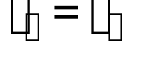
The identity function f(x)=x is often used as the output function:
|
However, other functions are not excluded. If the identity function is used as the output function, the distinction between activation and output functions is irrelevant. In the application of artificial neural networks, activation and output functions are often combined.
|
Company locations

Goldau |
|
|
Top Value GmbH 6410 Goldau |
|||
|
|
Phone: +41 (0) 41 552 11 30 |
|
|

Nyon |
|
|
Top Value Sàrl 1260 Nyon |
|||
|
|
Phone: +41 (0) 22 565 23 10 |
|
Top Value is dedicated to meeting the needs
|